Analysing data using Numpy

Overview

Teaching: 25 min
Exercises: 60 min

Questions

• How can I analyse data using Numpy?

• How can I fit a polynomial function to data?

• How can I apply mathematical operations to my data?

Objectives

• Fit a first order polynomial to data

• Access physical constants from the scipy library

• Apply mathematical and statistical operations across 1d and 2d arrays

In earlier tutorials we have read-in and plotted our raw transmittance spectroscopy data. In this tutorial we will analyse this data to calculate the band gap of each material. For our analysis we will make use of a number of functions in the Numpy library: numpy.polyfit, numpy.polyval and numpy.roots. We will also use Numpy array operations to calculate the reflectance of each material.

Digging a little deeper into transmittance spectroscopy

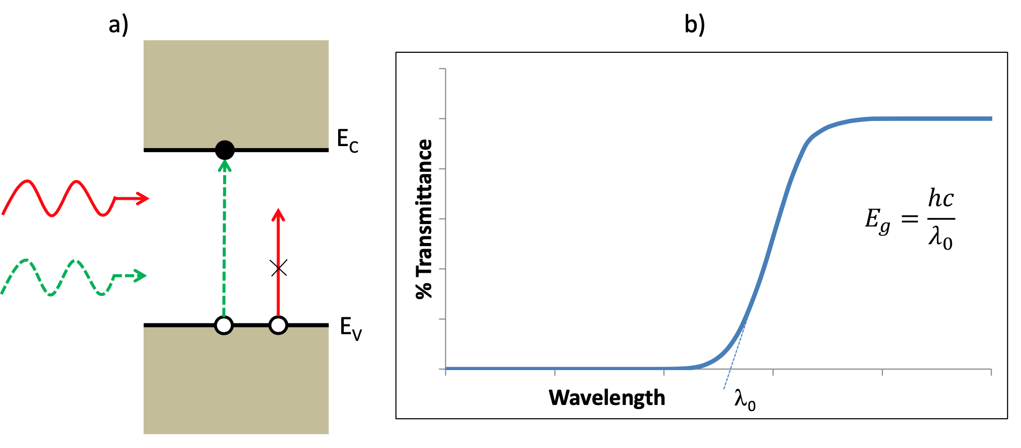
The schematic above is taken from the Lab script for course KD5081 at Northumbria University.

The optical transmittance spectrum of a semiconductor yields information on the energy band structure of the semiconductor. In particular if the frequency of the radiation $\nu$ is such that $E_g<h\nu$ where $E_g$ is the energy bandgap of the semiconductor then each photon absorbed creates an electron-hole pair and there is weak transmittance. If however $E_g>h\nu$ then the electron-hole pair cannot be generated and there is usually strong transmittance in this region. Thus by measuring the position of the transmittance edge, one can determine the energy bandgap of the material using the equation $E_g = h\nu = \frac{hc}{\lambda_0}$

It is, however, often difficult to locate the absorption edge precisely as it may be “smeared out” over a wide wavelength range. A simple criterion that suffices in this case is to take the point which is obtained by extrapolating the transmission curves. This requires a straight line fitting to the data, which will be our first analysis task.

There are often multiple ways to approach a programming task

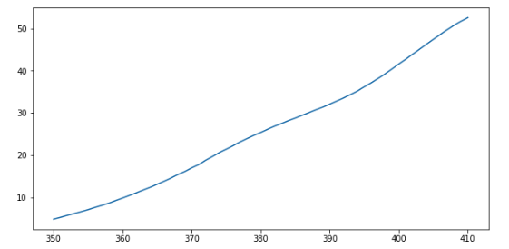
First we will slice our ITO transmittance data and visualise it to find the linear region. For example, the following slice generates a region that looks roughly linear.

plt.plot(wavelengths[50:111],ITO_transmittance[50:111],label='ITO')

We have done this manually, and “by eye”, but there are ways - beyond the scope of this course - to automate this process and reduce role of human judgement. For example, see this answer on the very useful site Stack Overflow.

Fit a polynomial function to data using the numpy.polyfit function

We can fit a polynomial to this data slice using the numpy.polyfit function. This function uses a least-squares method to perform the fitting. In this case, we know that is is a first order polynomial (straight line) - but note that least squares methods (and the polyfit function) can be used to fit higher order polynomials.

fit=numpy.polyfit(wavelengths[50:111],ITO_transmittance[50:111], 1)
print(fit)

array([   0.79366912, -275.85006769])

The polyfit function returns two values. From the function documentation (numpy.polyfit?) we can see that these are the polynomial coefficients with the highest power returned first. As this is a linear fit, the first value is the gradient of the line and the second value is the intercept on the y-axis.

We can overlay the fit on our dataset to verify that our fit is sensible. To do this we first evaluate this fit using the numpy.polyval function for a number of points along the x-axis.

fit_val = numpy.polyval(fit,np.linspace(350,410,1000)))

array([-6.00256795e+00, -5.94695550e+00, -5.89134305e+00, ...

This generates an array of y values.

We then plot the experimental data and our fit alongside each other. As there are now multiple plot lines we also include a legend.

plt.plot(wavelengths,ITO_transmittance,label='experimental data')
plt.plot(np.linspace(340,410,1000),fit_val,label='least squares fit')
plt.legend()
plt.title("ITO transmittance")

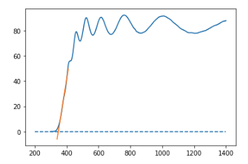
This looks sensible! To calculate the band gap energy of our material we need to calculate the point at which the fit intercepts with the x-axis. As our fit is linear, this point corresponds to the one and only root of our polynomial equation. To find the root(s) of a polynomial equation we can use the numpy.roots function.

lambda_0 = numpy.roots(fit)  # in nm
print(lambda_0)

[347.56306101]

Use the scipy.constants module for physical constants

To calculate the band gap we use the equation $E_g = h\nu = \frac{hc}{\lambda_0}$. This equation has two physical constants: h and c. We could hard code these values using scientific notation

h = 6.6e-34 # plancks constant
c = 3e8 # speed of light
lambda_0 = lambda_0*1e-9  # in metres
E_g = h*c/(lambda_0*1e-9) # E_g in joules
print(E_g)

[5.35154684e-19]

Alternatively we can import them as variables from the scipy.constants module - this is the preferred method as there is less chance of error.

from scipy import constants

E_g = constants.h*constants.c/(lambda_0*1e-9) # E_g in joules
print(E_g)

[5.71535379e-19]

The band gap is in joules. We will convert to eV as this is more commonly used for band gaps.

print(E_g*6.242e18)  # E_g in eV

[3.56752383]

Excellent! This falls within the band gap range reported in the literature.

Numpy simplifies and speeds up array operations

Arrays also know how to perform common mathematical operations on their values. The simplest operations with data are arithmetic: addition, subtraction, multiplication, and division. When you do such operations on arrays, the operation is done element-by-element. Thus:

double_ITO_transmittance = ITO_transmittance * 2.0

will create a new array double_ITO_transmittance each element of which is twice the value of the corresponding element in ITO_transmittance:

print('original:')
print(ITO_transmittance[:3])
print('double:')
print(double_ITO_transmittance[:3])

original:
[0.098 0.097 0.102]
double:
[0.196 0.194 0.204]

There are various ways to double the values in a Python list, but none are as elegant as the numpy syntax. For example, one way is list comprehension

double_ITO_transmittance = [x*2 for x in ITO_transmittance]
print('original:')
print(ITO_transmittance[:3])
print('double:')
print(double_ITO_transmittance[:3])

original:
[0.098 0.097 0.102]
double:
[0.196 0.194 0.204]

List comprehension syntax is compact but not as readable as the Numpy syntax. Furthermore, for large arrays, Numpy is faster.

If, instead of taking an array and doing arithmetic with a single value (as above), you did the arithmetic operation with another array of the same shape, the operation will be done on corresponding elements of the two arrays. Thus:

triple_ITO_transmittance = double_ITO_transmittance + ITO_transmittance

will give you an array where triple_ITO_transmittance[0,0] will equal double_ITO_transmittance[0,0] plus ITO_transmittance[0,0], and so on for all other elements of the arrays.

print('triple_ITO_transmittance')
print(triple_ITO_transmittance[:3])

tripledata:
[[ 2.38556340e-02  2.44810320e-02  2.51064270e-02 ...  3.00000000e+01
   3.89003241e+00  5.00009036e+00]
 [-8.07881400e-03 -7.33677000e-03 -8.08221000e-03 ... -3.67258608e-01
  -2.12232810e-02 -5.47421157e-01]
 [ 1.03191690e-02  1.11170400e-02  1.02593670e-02 ...  9.95927007e-01
   1.13159770e+00  1.06025667e-01]]

To calculate the reflectance R of the ITO we can use the formula $R = \frac{1-T}{1+T}$.

ITO_reflectance = (1 - 0.01*ITO_transmittance)/(1 + 0.01*ITO_transmittance)
print(ITO_reflectance)

[ 0.82149362,  0.82315406,  0.81488203, ..., -0.97743657,
       -0.97745971, -0.9774531 ]

There are Numpy functions for statistical analysis

Often, we want to do more than add, subtract, multiply, and divide array elements. NumPy knows how to do more complex operations, too. If we want to find the average absorption for all samples across all wavelengths, for example, we can ask NumPy to compute data’s mean value:

print(numpy.mean(ITO_transmittance))

75.42357584014532

mean is a function that takes an array as an argument. There are also numpy.min and numpy.max functions for calculating the minimum or maximum of an array.

Numpy functions can be applied across an axis

What if we need the mean transmittance for each material? In this case we use the whole data array and specify the axis we want to work on. In this case, we want the mean transmittance across each column (axis 1). We slice the data so as not to include the wavelength values in our calculation.

print(numpy.mean(data[:,1:], axis=1))

[850.          75.42357584  61.16855949  11.92739782   7.67069846]

If we wanted the mean transmittace for each wavelength, we are calculating the mean across each row (axis 0). Again we slice the data so as not to include the wavelength values in our calculation.

print(numpy.mean(data[:,1:], axis=0))

[ 0.0635   0.0635   0.06575 ... 58.4015  58.53025 58.62425]

Error bars and exponential growth

This question is partly modelled on the a blog post. There is also a nice 3Blue1Brown video on exponential growth in the context of Covid.

We have the following (hypothetical) data for the number of Covid cases at a university over a two-week period: 3, 4, 8, 15, 32, 65, 128, 253, 512, 1025, 2049, 4090, 8191, 16387. Each data point corresponds to the positive test results received on a single day.

Create a one-dimenstional Numpy array to hold this data. Scatter plot the data and save as a .png file. Save the raw data to a .csv (comma separated variable) or .txt file.

Solution

import numpy as np
import matplotlib.pyplot as plt

case_numbers = np.array([3,4,8,15,32,65,128,253,512,1025,2049,4090,8191,16387])
plt.scatter(np.arange(0,15),case_numbers)
plt.xlabel("Day number")
plt.ylabel("Covid case count")

plt.savefig("Covid_case_numbers_plot.png")
np.savetxt("Covid_case_numbers_data.csv", case_numbers, delimiter=",")

An administrator realises that some test results may have been filed a day late or a day early. This makes the error bar on the case numbers +/- 200. Using the matplotlib.pyplot.errorbar function with the yerr keyword argument plot the case number data with error bars. Label your axes and title the plot.

Solution

import matplotlib.pyplot as plt

plt.errorbar(day,case_numbers,yerr=200)
plt.xlabel("Time (days)")
plt.ylabel("Case numbers")
plt.title("Covid case numbers over time")

By taking a logarithm of the data, fit a straight line to the case number data and predict the exponential growth factor.

Solution

From scanning the blog post we can see that the growth factor is the base of the exponential. Assuming the growth is exponential, to generate a straight-(ish) line we first need to take a logarithm of the case values data. We can then fit a straight line to this to calculate the logarithm of the growth factor.

log_growth_factor, log_starting_case_number = np.polyfit(day,np.log(case_numbers),1)
growth_factor = np.exp(log_growth_factor)

From inspecting the data, does the calculated growth factor make sense?

Solution

The data roughly doubles each day. The calculated growth factor is 1.94, which is reassuringly close to 2.

Calculating the band gap of photovoltaic materials

In the tutorial we calculate the band gap of ITO. Following the same procedure, calculate the band gap of one of the following photovoltaic materials: CdS, Si or GaAs. To verify your code compare your band gap value to those found in the literature

Encapsulation

If you want to repeat the same analysis step(s) a number of times you may want to write a function. Fill in the blanks to create a function that takes a single filename, containing comma separated values, as an argument, loads the data in the file named by the argument, and returns the minimum value in that data.

import numpy

def min_in_data(....):
    data = ....
    return ....

Solution

import numpy

def min_in_data(filename):
    data = numpy.loadtxt(fname=filename, delimiter=',')
    return data.min()

Key Points

• There are often multiple ways to approach a programming task

• Fit a polynomial function to data using the numpy.polyfit function

• Use the scipy.constants module for physical constants

• Numpy simplifies and speeds up array operations

• There are Numpy functions for statistical analysis

• Numpy functions can be applied across an axis